GWV offers tools for trial and error as well as automated calibration
- We will use 16 head target locations
- The data could be entered one at a time through the interface
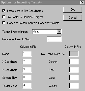
- But we will import text file containing the target data
- Select Add->Import->Targets
- Select targets.dat
- Click OK
- In this case, the default values for file format are correct, so look them over to become aware of the options/issues,then
- Select OK
16 targets will appear on the plan view as small blue dots- 6 in layer 1, 5 in layer 2, and 5 in layer 3
- You may edit target information in Analytic Element mode by double-clicking on a target symbol
- Model results must be imported again to compute the calibration statistics
- Select Plot->Import Results
- Click OK
- Select Plot->Calibration->Statistics/Plots…
- Select the type of targets to use in the calculation and ranges of layers
- Click the Statistics button and review the items in the list
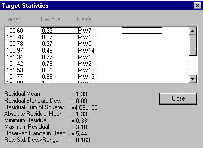
Click OK- Click the Plot Observed vs. Simulated button
- Targets are color coded by layer
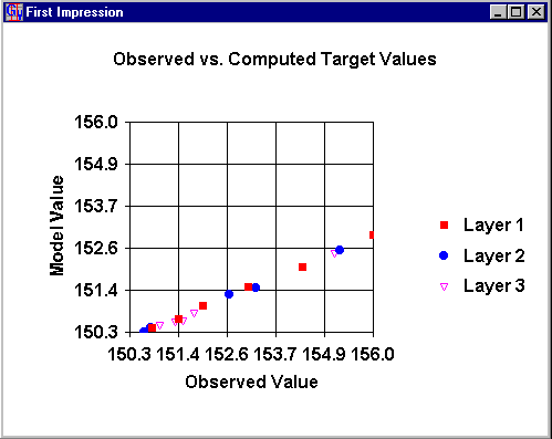
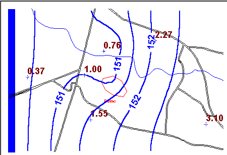
Notice the strong bias such that higher heads are simulated too low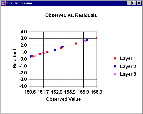
Notice all of the residuals are positive- To post residuals on a contour map
- Select Plot->Calibration->Post Residuals
- Check Post Residuals
- Change the font size by selecting Plot->Calibration->Target Options
- Click the font button to change the size or font
- Select View->Refresh to redraw
- Turn off the grid display by selecting Plot->What to Display
- Uncheck the option for finite-difference grid
- For layer one:
Sensitivity analysis is the process whereby model parameters or boundary conditions are altered slightly and the effect on model calibration statistics is observed- You choose a parameter type, the number of simulations, and a parameter multiplier for each simulation
- GWV then runs MODFLOW the desired number of times and produces a sensitivity plot
- Calibration statistics versus parameter multiplier are displayed to show Select Model->AutoSensitivitySetup
- Select Kx as the parameter to vary
- Keep the default of Zone number 1 and 5 simulations
- Click Multipliers and Enter 0.2, 0.5, 1.0, 1.5, and 2.0 for simulations 1-5
- OK
- Select Models->RunAutoSensitivity
- Yes to view results
- View the sum of squared residuals, residual mean, residual standard deviation, average drawdown, and total flux to a designated boundary condition reach ... sum of squared residuals are shown
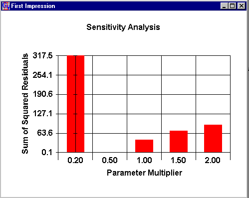
Notice a Kx value of half the current value gives a much better calibration- GWV also supports AUTOMATED CALIBRATION through PEST, UCODE, and MODFLOWP
- Select Model->Calibration
- Select the parameters that you would like to estimate
- We will estimate horizontal hydraulic conductivity in zone 1 (which is the whole model in this case)
- Select Model->Calibration->Parameters and enter the data shown on the following dialog
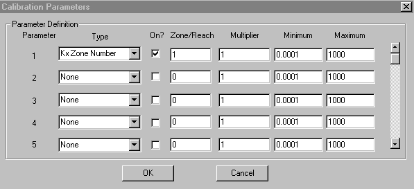
GWV estimates a multiplier on the parameter value so the multiplier of 1.0 in column 4 above means that we will start with our initial guess (in this case 100 ft/d).- The minimum and maximum values constrain the parameter value. These are also multipliers.
- Now select Model->GVCalibration->Options and change the number of iterations from 25 to 5
- Click OK
- Select Model->GVCalibration->Start Calibration
- MODFLOW will run a number of times
- If the model does not converge on some executions, allow it to continue anyway
- If you are asked, say YES to look at the calibration summary each time
- If you are asked, Continue to save parameters for next iteration and continue to next iteration until the values no longer change and the optimal solution has been found
- When the calibration is complete
- Notice how the value of Kx has changed (the multiplier reflects this)
- Notice that the optimal value (0.5) was found quickly and most of the effort was necessary
- Notice how the statistics have changed
- If you like the results of the calibration run,
- Select Model->GVCalibration->EndCalibration if you haven't reached the last iteration
- Select Model->GVCalibration->Update Databases
- This command takes the results of the calibration and puts the new values in the data base
- Rerun the model for one simulation to make sure your MODFLOW files contain the new values
- View the reduced and balanced residuals
- Automated calibration does not always go smoothly
- Estimate as few parameters as possible and only sensitive parameters
- If GWV Calibration does not work try one of the more robust calibration tools such UCODE, PEST, or MODFLOWP.
- The data could be entered one at a time through the interface