1. Initial material properties and boundary conditions must be consistent with the initial heads. If you start with initial heads that are contoured from field measurements and you do not apply a stress to the system, the heads will adjust to the properties and boundaries, so you are inadvertently introducing a stress by defining inconsistent values for starting conditions. The most common way to deal with this problem is to calculate a pre-stress steady state solution for use as initial heads.
2. If the field system being simulated is not in equilibrium, an earlier equilibrium condition can be identified and defined as a starting point. All subsequent stresses must be simulated from the time when equilibrium prevailed until time when the initial conditions are needed is reached, then the early stresses must continue along with the new stress of interest if the early stresses continue in the field.
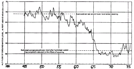
A classic example is this hydrograph of a well on Long Island displaying the impact of sewering which started in the mid 50's and was completed in mid-60's.

The upper dashed line represents a long term steady state condition. There are daily and seasonal variations but the average values are relatively constant in time. The lower dashed line represents the new long term steady state condition that prevails after the full impact of sewering has been realized.
The water levels decline as a result of sewering because recharge that used to enter the ground water via septic tanks is now routed away by the sewers.
Suppose you wanted to simulate the impact of a proposed municipal water supply well that would go on line in 1962. In order to obtain a consistent set of starting values for initial conditions in 1962, it would be necessary to simulate the early equilibrium that prevailed until 1955, add the stress of the gradually reducing recharge in space through time until reaching 1957, then continue simulating the reductions in recharge along with the addition of the pumping well.
It is vital that you develop hydrographs of an area and come to understand these transitions before undertaking an elaborate modeling project.
Another item to note while viewing this diagram is this. If you had water level data from a number of wells prior to 1955, the average of those values would reflect the average water levels during the early period for one set of boundary conditions and stresses. However if data from 1950 through 1975 were mixed together and averaged, the result will NOT reflect a set of boundary conditions and stresses that occurred together in the field.
3. What can we do if we cannot use a steady state initial condition because our problem is dependent on a short term response during a particular time of year? In this case there may be a quasi-cyclic equilibrium in the area, that is a general repetition of conditions that occur year after year and we may attempt to represent that situation, then start our stress at the appropriate point in the cycle. Draw diagrams of the variations and the timing of your stress and coordinate this with a diagram of model stress periods and time steps to help yourself get everything timed correctly in your model.
4. What if we do not have sufficient data to establish an acceptable steady initial condition to commence our cyclic equilibrium? In this case, we may be able to start with a rather arbitrary initial condition but simulate the cycle long enough such that we simulate the same values at the same times in subsequent cycles.
5. It may be that there is enough information in your transient data to estimate initial conditions. This can be judged by evaluating the sensitivity of initial conditions to the available data and the correlation of parameters defining those conditions to other parameters that are estimated.
6. Finally, it is useful to note that the further, in time, the simulation is from the initial conditions the less influence those initial conditions have on the simulated values.
7. Recall the procedure for discretizing time as discussed in Unit 7.
Now lets
explore the transient character of the MODFLOW problem that we have been using
as a class example. By undertaking a transient modeling exercise involving variable
recharge and pumping.
Click here to undertake the transient exercise
GO "BACK" to the transient main page