EXERCISE 7b: Execute a Transient Model of the Pumping with Variable Recharge

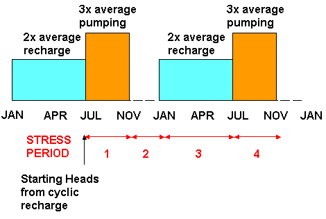
Start at the end of a "wet" period, the end of June
Define 4 stress periods:

Jul-Oct (4mo) = no recharge, pumping

Nov-Dec (2mo) = no recharge, no pumping

Jan-Jun (6mo) = high recharge, no pumping

Jul-Oct (4mo) = no recharge, pumping

1. Save ex7a in a directory ex7b as ex7b.gwv use a root file name of extr7b

Confirm that the paths to models are correct

2. Specify stress periods

Model>MODFLOW>BasicPackage

Specify 4 stress periods

Model>MODFLOW>StressPeriodSetup

Jul-Oct = (4mo) 1.0512x10⁷ sec

Nov-Dec = (2mo) 5.256x10⁶ sec

Jan-Jun = (6mo) 1.5768x10⁷ sec

Jul-Oct = (4mo) 1.0512x10⁷ sec

use 10 steps each and multiplier of 1.1

Model>MODFLOW>InitialHeads

Select extr7.hds from ex7a

stress period 29, time step 10

3. Set output controls

Model>MODFLOW>Output Control Package

Save heads every tenth time step to have them at the end of each stress period

uncheck the Disable printing box

Models>MODFLOW>PrintFormats

print all relevant items for your problem

4. Edit properties

With Edit mode set for properties

Step through the stress periods and set the RCH for the zone near the river as 4x10^-8 and the zone away from the river as 2x10^-8 for period 3; all other recharges should be zero

With Edit mode set for BC

Replace the wells in each layer and set transient pumping rates at 3cms for stress periods 1 and 4
Notice that you need to uncheck steady state and select Transient Data to input stress period 1 to1, -3; 2 to 3, 0; and 4 to 4 -3

Remember to include the well package in the model

GHBs and RIVs need not be considered because the default is that boundary conditions are steady unless specified otherwise

5. Run MODFLOW

Create MODFLOW files

View the new bas, wel, rch, and oc files

Execute MODFLOW

View results by comparing profiles in row 9 and model budget summaries at the end of each stress period

FIRST! Check the recharge and well files to see how they have changed
Also: Peruse the MODFLOW output file, looking for conditions that you do not expect

Look at the Model Mass Balances and Head Profiles along row 9 at the end of each stress period:

Stress Period 1: Notice the extreme drawdown after 4 months of pumping during the dry period

Stress Period 2: Notice that once the pumping stops, the river recharges the system
This may bring to mind the issue of how much water is being withdrawn from the river? We do not know the flow rate of the river but we may find that there is not enough water available to support the river seepage calculated by the model.
If we found that there was sufficient river discharge to supply this volume of water what might we propose?answer

Stress Period 3: Notice, after the wet season the basin is nearly fully recovered

Stress Period 4: The second pumping cycle yields nearly similar conditions as the first indicating a cyclic (albeit physically impossible) equilibrium has been reached for the new recharge/pumping cycle

6.Consider the significance of these results

BE WARY! NOTICE WHAT MODFLOW ISN'T TELLING YOU

What type of prediction would you make from these results? answer

Why did everything look fine when we used average annual rates, and it doesn't look fine now? answer

It will not take long to make these layers convertible and rerun the problem. Remember to establish a new cyclic equilibrium given the convertible condition before beginning the scenario of pumping during the dry season. Try that now. Resulting files are not provided. Email me if you have trouble accomplishing this.

The transient exercise is complete, GO "BACK" to the home page for unit 11 to complete the unit.