For now consider TRIAL-AND-ERROR CALIBRATION involving:
An effort to minimize residuals, where a residual is the difference between a measured value observed in the field and the equivalent value simulated by a model:
When calibrating a model one strives to achieve:
1) A similarity of measured and simulated conditions through steps 2 through 6.
2) Minimum global measures of error such as:
The Mean Error:

However use of the Mean Error can be misleading because large negative and positive residuals can cancel. The Mean Absolute Error prevents negative and positive deviations from canceling out in the global measure:

The Root Mean Squared Error prevents negative and positive deviations from canceling out and emphasizes large deviations in the global measure:

Similarly the Sum-of-Squared Weighted Residuals prevents negative and positive deviations from canceling out, emphasizes large deviations, includes a weight on each residual to reflect the certainty associated with the field measure, and is often used as the value to be minimized for calibration:

- WEIGHTING RESIDUALS:
- The nature and level of certainty associated with observations may vary, so we weight residuals before making the above measures of error, typically:
- Weight = w = 1 / (measurement variance)
- And we use weighted residuals (using w0.5 as the weight) or weighted squared residuals (using w as the weight) in the above evaluations
- If numerous measurements are not available for calculation of the measurement variance, we can determine the variance as follows:
Make an estimate of your certainty associated with the measurement. For example, there is a 95% probability that I am measuring the flow rate of 300cfs to within +/- 30cfs. Once you formulate such a statement, you can determine the standard deviation by noting from any table of the normal distribution (in any basic statistics book) that a 95% probability is equivalent to 1.96 standard deviations, thus:


- Notice, when the squared residual is multiplied by the weight, the resulting weighted squared residual is dimensionless. This means that it is possible to mix observations with different types of units.
- The nature and level of certainty associated with observations may vary, so we weight residuals before making the above measures of error, typically:


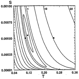
From here, extend the concept to think about working your way to the lowest point on the surface. Once you have more than 2 or 3 parameters the surface cannot be visualized physically, but the idea is the same: seek how the parameter values must change to reach the lowest point on the surface (i.e. minimize the SOS). That is, we need to know: which way does the surface slope and at what magnitude (sensitivities), and how far are we from the minimum (residuals)? Then we need to adjust the parameter values to reach the minimum. Of course the surface is controlled by the conceptual model and the model construction. Generally discussion of calibration does not include adjustment of these values, but it should. Automated calibration focuses the modeler on this aspect of calibration an then uses nonlinear regression to find the optimal parameter values for that model setup.
3) COMMON SENSE I can't write an equation for that!
4) Graphical measures of error
- ymeasured vs. ysimulated which is
expected to form a 45o line passing through the origin

- residual vs. ysimulated which is expected to form
a uniform horizontal band centered on zero

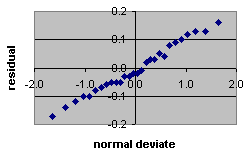
- probability distribution of residuals which should form a
straight line on probability paper

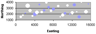
- Map (ymeas - ysim) in x, y, z space
should exhibit a random pattern of positive (white) and negative (blue), as
well as large and small, residuals

- Graphs of (ymeas - ysim) vs. time OR
vs. observation # should form a uniform horizontal band centered on zero

Targets are sometimes used for trial-and-error calibration.
- Targets may have different ranges reflecting the uncertainty
associated with the observation (note: being within target range is as good
as on target)
- Level 1 = within measurement/model error
- Level 2 = within 2x that error
- Level 3 = within 3x, etc.
- Level 2 = within 2x that error
- Target levels are plotted on a map of an area, generally with a symbol proportional to the target level.
- Level 1 = within measurement/model error