To illustrate the concepts of transient modeling, we will add a pumping well to the system that we worked with previously, continuing from exercise 4b. The well is located at x=9500, y=9500, the center of row 9 column 10, and is believed to be pumping an average of 1 cms in both layers We will use the heads from the steady state model without pumping that we have been using for class exercises as the starting heads for the transient simulation

IF YOU DID NOT SET UP THE GWV FILES FOR THE PROBLEM PREVIOUSLY USED AS AN EXAMPLE, then either do so now, or download the gwv file and save it to a location that is appropriate for exercise 5.

First, unless the steady state occurrence of the transient stress is a physical impossibility, one should always begin by making a steady state simulation of the stress THIS WILL REVEAL THE MAXIMUM IMPACT ON THE SYSTEM

We will continue from exercise 4b where we had an 18x18x2 grid with a river and general head boundary package.

Then move on to: Exercise #5

Once the ultimate steady state condition is known, we start the pumping scenario from the steady state heads under pre-pumping conditions as initial conditions and proceed to simulate the transients.

If you were editing files with a text editor and running MODFLOW, you would refer to the binary heads in exss.shd in the BAS package of the transient run (binary heads are entered by indicating a negative unit number). The unit number would correspond with the unit number specified for exss.shd in the name file.

You will have to determine how to get the initial heads into the GUI that you choose to use.

I will use GroundWater Vistas to demonstrate the transient modeling exercises.

To initiate a transient run, the following tasks need to be done:

BAS: initial heads, stress periods & time steps need to be defined

BCF: storage properties need to be added

WEL: the stress needs to be defined

Packages that represent stresses (e.g. RCH, GHB, & RIV) need to be visited to either, define how the stress changes with each stress period, or to state that it remains the same as the previous period

Output Control Options need to be defined for the Stress Periods

Now move on to: Exercise #6

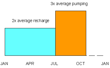
Consider now, that the recharge is variable:

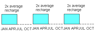
It is twice the average rate we used for the steady state case from January through June and zero for the rest of the year.



Now also assume that the pumping occurs at three times the rate we used as an average, but for only a third of the year, from July through October.



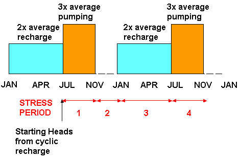
Let us determine what conditions are like after two pumping seasons.

We will need to add more stress periods.

First we need to establish initial conditions, so we run a model without the well (remove the well package) AND run with cyclic high and low recharge, for enough cycles such that conditions at July 1 are the same as the previous year, so ....

Proceed to: Exercise #7a

Once initial conditions are established we can evaluate the transient situation:



In: Exercise #7b

GO "BACK" to the transient main page