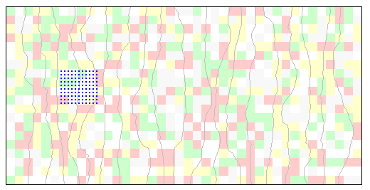
Open the web page, Sample Random Walk Simulation read the brief directions, then follow these steps
-
- Start:
- Grid Spacing
50
- Columns 20
- Rows 40
- Average gradient 0.001
- OK
- Columns 20
- Check Randomize
- OK
- 20
- Compute
- Check Particle Movement
- Initial Particle Spacing 20
- OK
- Initial Particle Spacing 20
- Click the left mouse button 4 times
forming a square, and holding the shift key while clicking the 4th time
 Animation
- 1 sec 30 days
- Longitudinal Dispersivity 10
- Transverse Dispersivity 5
- Check Show Center of Mass
- OK
- Longitudinal Dispersivity 10
- Click again to stop/start particles
Notice the particles "jump" in a forward advective step, but then the random movement of the dispersive step make the particles move backwards at times as well as sideways.
Notice the net effect of the plume with time
You can lay any size grid over this and compute concentration as the number of particles times their mass divided by the volume represented by the grid
A coarse grid causes averaging of the concentration
A fine grid provides a more accurate reflection as long as it is not so fine such that many of the grid cells contain no particles.
The local velocity controls the advective step, so if the time step is long you will miss the twists and turns of the flow lines as they adjust to the heterogeneity
Recall that dispersivity is a construct of the hydrology profession to cope with variable advection at a scale that is too small to represent with flow models
You can experiment with comparing random walks through homogeneous materials with various values of dispersivity to heterogeneous models with ZERO dispersivities
CLOSE the RANDOM WALK MODEL- CLOSE the external WEB PAGE
- GO "BACK" to continue exploring solution techniques for contaminant transport simulation
- Start: