Steady-State Topography-Driven Flow
Developed by Paul Hsieh, USGS
Skip ahead to run the model
Introduction
A topography-driven flow system is one in which ground water flows from higher-elevation recharge areas (where hydraulic head is higher) to lower-elevation discharge areas (where hydraulic head is lower). See figure below.
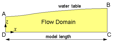
The boundaries of the flow domain are as follows:
- The top boundary (AB) is the water table, which is assumed to lie close to land surface.
- The two vertical boundaries (BC and AD) are no flow boundaries.
- The bottom boundary (CD) is also a no-flow boundary.
The no-flow boundaries might represent low-permeability bedrock that bounds the basin. Alternatively, the vertical boundaries might also represent ground-water flow divides. Important Note: By specifying the position of the water table, it is assumed that the pattern of recharge and discharge is such that the water table is maintained at steady state.
Governing Equation
The steady-state ground-water flow equation to be solved is
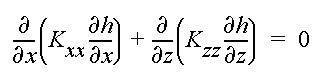
where h is hydraulic head, and Kxx and Kzz are the principal values of the hydraulic conductor tensor. The principal directions are assumed to be parallel to the xand z axes.
Boundary Conditions
Assuming we know the position of the water table, the boundary condition along the water table (AB) is

where z is the elevation of the water table.
Along the vertical boundaries BC and AD, the no-flow boundary condition is

Along bottom boundary CD, the no-flow boundary condition is

After solving for hydraulic head h, the x and z components of the linear velocity vector are computed by
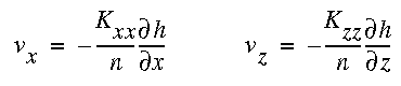
where n is porosity. The velocity vectors are used for calculating flow paths and the advective movement of fluid particles.
Running the Model
Running the model involves 7 steps. To begin each step, click the corresponding button at the top of the window. A dialog box appears for you to enter the necessary input data. The three buttons on the second row allow you to zoom in, zoom out, and quit the model.
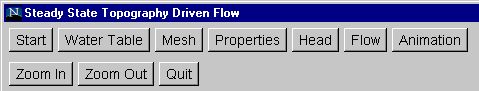
Step 1: Start -- Specify model dimension
Step 2: Water Table -- Specify the position of the
water table
Step 3: Mesh -- Specify the dimension of the model mesh
Step 4: Properties -- Specify hydraulic conductivity
and porosity
Step 5: Head -- Compute hydraulic head
After hydraulic head is computed, two options are available. You may proceed to
Step 6a: Flow (Path) -- Track flow paths from selected
points
Step 7a: Animation -- Animate the evolution of flow
paths
or
Step 6b: Flow (Particle) -- Set up initial distribution
of fluid particles
Step 7b: Animation -- Animate the advective movement
of fluid particles
Updated on July 11, 1999.