Eileen P. Poeter, Corresponding Author
Department of Geology and Geological Engineering
Colorado School of Mines
1500 Illinois St.
Golden, CO 80401 USA
phone: (303)273-3829
fax: (303) 273-3859
email: epoeter@mines.edu
Mary C. Hill
United States Geological Survey, Water Resource Division, Box 25046 MS 413, Lakewood,
Colorado, 80225, United States of America
While for some constructed models the parameter estimation is unique, the overall model calibration is never unique for the complicated ground-water systems commonly considered. In practice, multiple constructed models must be developed at the beginning of a project and, depending on the character of the incoming data and results of ongoing analyses, each model is either retained for further consideration or eliminated during the modeling process.
Parameter estimation can be approached using an inverse model (Poeter & Hill, in press); for example, nonlinear regression can be used to find the set of parameter values that provides the best fit of model results to field observations, where "best fit" is defined as minimizing the value of the sum-of-squared weighted residuals. However, parameter estimation is often accomplished by a trial-and-error approach, during which the modeler iteratively selects parameter values to improve the fit of model results to field observations using intuition about model response to changes in parameters, and knowledge of reasonable parameter ranges. The time consuming nature of intuitive parameter value adjustment limits the range of alternative constructed models that are considered and, given the lack of rigorous analysis of parameter correlations, variance/covariance, and residuals, there is no assurance that the estimated parameter values for any model are 'the best'. Consequently, conclusive model discrimination is nearly impossible. This shortcoming is often so extreme that only one constructed model is considered. With inverse models used to determine parameter values that optimize the fit of the model results to the field observations for a given model configuration, the modeler is freed from tedious trial-and-error calibration involving changes in parameter values so more time can be spent addressing insightful questions about the hydrologic system.
If a constructed model is not an adequate representation of the ground-water flow system, then the estimated parameter values are not likely to reflect field conditions, predictions made using the model are likely to be in error, and decisions based on those predictions may not produce the best, or even a reasonably accurate, result. Indicators of inaccurately constructed models also include non-random weighted residuals and poor fit to the data, but the indicator focused on in this work is unreasonable parameter values (e.g. a lower hydraulic conductivity for a sand than a clay, or a boundary flux with the wrong sign) yielding the best fit between the observed and simulated values (such as hydraulic heads, concentrations, and flows). Thus, during calibration it is important to determine if the best model fit is achieved for unreasonable parameter values and whether these parameter values are well estimated with the available data.
Best-fitting unreasonable parameter values are more likely to be discovered using the inverse modeling approach than by trial and error, because the inverse model will determine the parameters that provide the best fit even though they may be of unreasonable absolute or relative magnitude. A modeler using the trial-and-error approach generally will not try unreasonable values (e.g. a much higher hydraulic conductivity for a silt deposit than an adjacent sandy-gravel deposit). Instead, usually unknowingly, the modeler accepts greater discrepancies in the match between field observations and model results (i.e. sacrifices the best fit between the model and the data) to maintain reasonable model parameters.
The output of unreasonable values is often disillusioning to new users of inverse models, but it is actually a great benefit. At first glance it may seem that the trial-and-error approach provides the more reasonable result and so would be the preferred method. However, when the modeler sacrifices honoring data to maintain "reasonableness", important information about the system is ignored and evidence of error in the constructed model is not allowed to surface. It is our experience that well estimated, unreasonable parameter values produced by the inverse model indicate that the constructed model is incorrect. With this information and the statistics calculated by the inverse model, the modeler can call upon experience with the geohydrologic systems and knowledge of reasonable parameter values to develop and test numerous constructed models, increasing the likelihood that accurate models will be used for prediction.
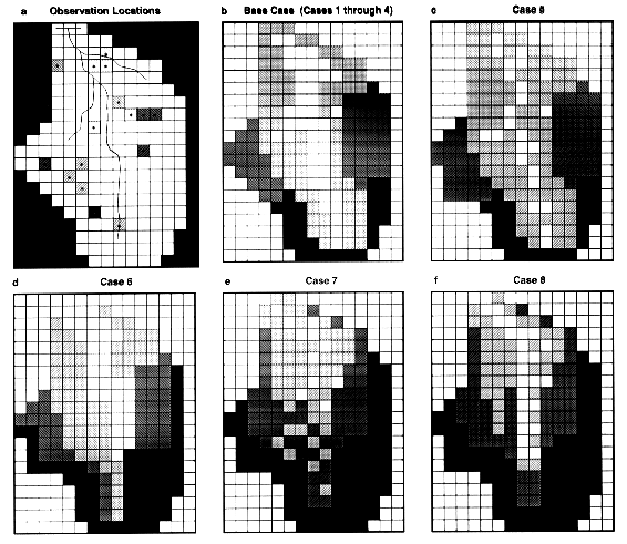
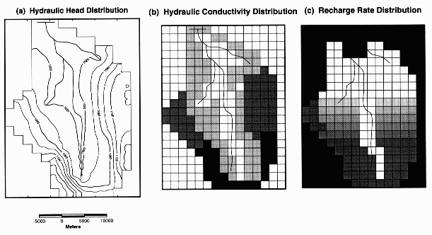
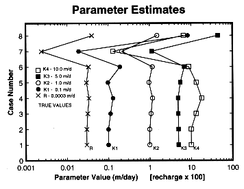
For this simple basin model, the hydraulic conductivity value of the four hydrofacies (K1-K4) and the magnitude of the recharge R (given its relative spatial distribution) are estimated. Hydraulic conductivity distributions and estimated parameter values for the following cases are presented in Figs. 2 and 3 respectively.
Case 1 - the base case: with error-free observations, a perfect constructed model, and correct "true" values of parameters as a starting point, the parameter estimation process quickly converges on the true parameter values (Figs. 2b and 3).
Case 2 - incorrect initial estimates: with error-free observations, a perfect constructed model, and incorrect initial values of the parameters including various combinations of parameters defined as two of orders of magnitude too small or large, the parameter estimation process quickly converges on the true parameter values (Figs. 2b and 3).
Case 3 - error in observations: with error-laden observations having normally distributed noise with a standard deviation of 2 m on the head observations and the flow underestimated by 4%, a perfect constructed model, and true parameter values for initial estimates, the code converges readily to values near the true values. The estimated parameter values are slightly different than the true values, reflecting parameter values that better fit the erroneous observations (Figs. 2b and 3).
Case 4 - larger error in observations: identical to Case 3, but with a standard deviation of 4 m on head observations and a flow measurement underestimated by 7.5% (Figs. 2b and 3).
Case 5 - minor zonation error #1: with error-free observations and accurate initial values for the parameters, a more discontinuous definition of the coarsest-grained (high hydraulic conductivity) zone than exists in the Base Case (Fig. 2c) results in rapid convergence on parameter values close to the correct values (Fig. 3).
The cases presented to this point pose some formidable problems to the parameter estimation algorithm without difficulty in obtaining reasonable estimates. The remaining two cases show how larger errors in the facies zonation pattern can create large errors in the estimates of parameter values.
Case 7 - major zonation error: when the percentage of fine-grained facies (K1) is substantially over estimated and the percentage of coarse-grained facies (K4) is underestimated and is much more discontinuous than in the base case (Fig. 2e), an unsatisfactory set of parameter estimates results. All of the parameters, including recharge rate, are estimated to be nearly an order of magnitude or more lower than the base case values. The estimated K of the coarse-grained facies is lower than the medium grained facies (Fig. 3).
Case 8 - major zonation error: sometimes the predominant geology in a small borehole is not thought to represent the geology of a 4x10⁶ m2 flow model grid block, so this variation includes three locations where the geologic observations are not honored for the flow model grid block (Fig. 2f) and yields a more reasonable recharge rate, but overestimates the K of the three finest-grained facies. The relative order of hydraulic conductivity between facies is again incorrect with the finest-grained facies exhibiting a higher hydraulic conductivity than the coarsest-grained facies and a reversal in the expected Ks for the two coarsest-grained facies (Figs. 3).
Using the model construction described by LeBlanc (1984), it was found that the best fit to the advective travel, head, and flow data was achieved with reasonable parameter values except for the areal recharge rate, which was about half the expected rate. In addition, the recharge rate was estimated precisely enough that a linear 95-percent confidence limit interval constructed about the estimate did not even come close to including reasonable values. This indicates that the data used are sufficient to distinguish between an accurate and inaccurate model, and that the constructed model was significantly inaccurate in some way. A variety of potential model construction problems that might cause the unrealistic recharge rate were tested by using regression to find the best-fit parameter values in each case. One of the considered alternatives proved to be a plausible explanation of the problem; it involved the constant-head boundary condition imposed along the southern boundary and southern parts of the east and west boundaries of the model. These boundaries represent surface-water bodies. The elevations of the surface-water bodies were derived from 10-ft contour topographic maps, and these elevations were used as the defined head at these boundaries, as is common practice in the development of ground-water models. It was found that if these 'measured' heads were consistently higher (by just one foot) than the surface-water body levels when the hydraulic heads used in the regression were measured, the estimated recharge rate would be about half of a reasonable rate. This indicates that, in systems such as this in which surface-water bodies define boundary conditions through which most or all of the water flows, and ground-water levels are only on the order of 5 ft above the surface-water bodies, it is important to accurately measure the elevation of the surface-water bodies at the same time as ground-water heads are measured.
The plausibility of each stochastic hydrofacies zonation was determined via parameter estimation using MODFLOWP. Use of soft data, coupled with elimination of realizations when parameter estimation revealed a poor fit and/or unreasonable parameter values, resulted in narrower confidence limits on the estimated values. This sensitivity to fine scale, geologically based zonation patterns is fortunate because it allows use of hydraulic-head data and prior information on reasonable parameter values to delineate the small scale heterogeneity that is critical to the migration of contaminants and reduces the uncertainty associated with predicted flow through the site.
Anderman, E. R., Hill, M. C., & Poeter, E. P., 1996, Two-dimensional advective transport in groundwater flow parameter estimation, Ground Water, Vol. 34, No. 6., pp. 1001-1009.
Barlebo, H. C., Hill, M. C., & Rosbjerg, D. in review, Three-dimensional inverse modeling using heads and concentrations: Application to a Danish Landfill, submitted Wat. Resour. Res.
Christiansen, Heidi, Hill, M. C., Rosbjerg, Dan, & Jensen, K. H. 1995, Three-dimensional inverse modeling using heads and concentrations at a Danish Landfill, Wagner, B., and Illangesekare, T., eds, Models for assessing groundwater quality, IAHS Pub. no. 227, pp. 167-175.
Hill, M. C., Cooley, R. L., & Pollock, D. W. in review, A controlled experiment in ground-water modeling, 1: Inverse modeling with nonlinear regression and parameterization: submitted Wat. Resour. Res.
Hill, M. C. in review, A controlled experiment in ground-water modeling, 2: Evaluation of first-order measures of prediction uncertainty: submitted Wat. Resour. Res.
Hill, M. C. 1992, A computer program (MODFLOWP) for estimating parameters of a transient, three-dimensional groundwater flow model using nonlinear regression: USGS OFR 91-484, 358p.
LeBlanc, D. R. 1984, Digital model of solute transport in a plume of sewage contaminated ground water: in LeBlanc D. R., ed. 1984, Movement and fate of solutes in a plume of sewage-contaminated water, Cape Cod, Massachusetts. U.S. Geological Survey Open-File Report 84-475.
McKenna, S. A. & Poeter E. P. 1995, Field Example of Data Fusion for Site Characterization, Wat. Resour. Res. 33 (6), 3229-3240.
Poeter, E. P. & M. C. Hill, in press, Inverse models: A necessary Next Step in Groundwater Modeling, Ground Water.
Poeter, E. P. & McKenna, S. A. 1995, Reducing uncertainty associated with ground-water flow and transport predictions, Ground Water 33(6), 899-904.