Image processing for faults
August 1, 2014
I am writing this note while travelling to Australia in the first leg of a worldwide lecture tour for the Society of Exploration Geophysicists. I am super excited to be doing this, for some obvious reasons, but also because this tour gave me a perfect excuse for new research of seismic image processing for geologic faults.
- Vertical slices of a 3D seismic image, before and after unfaulting.
The 3D seismic image of the onshore Schoonebeek oil field in the Netherlands was provided by Kees Rutten and Bob Howard, via TNO, a Dutch research organization. It's a geologically beautiful high-resolution image, with numerous intersecting faults. Displayed above are vertical slices of this 3D seismic image, before and after unfaulting. The vertical white line represents the intersection of orthogonal vertical slices through the 3D image.
The methods for locating faults and estimating fault slips are entirely automatic, and consist mostly of some well-known image processing techniques combined in ways that I describe in the SEG lecture.
Unfaulting here does not imply a reversal of geologic time, a restoration of the subsurface to some original unfaulted state. Rather, unfaulting is a simple way to assess the accuracy of the estimated fault locations and slips. After unfaulting, subsurface reflectors should appear more continuous, and this increased continuity is clearly apparent. But not everywhere, and shortcomings are opportunities for future research.
One shortcoming is that the footwall side of every fault has been constrained to not move during unfaulting. Where faults intersect, this constraint leads to some kinky unfaulted seismic reflectors. These do not affect our visual assessment of estimated fault slips, but how might we do better?
While thinking about that question, you can test this processing with your own 3D seismic images, because all of the image processing software used here is freely available with an open-source license. That license enables companies to use this software in commercial software products. Some have already done so, because an earlier version (now about two years old) has been available with the same open-source license.
If you download the latest version, note that it includes software for generating synthetic 3D images for testing. You can modify this software to answer some good questions. For example, what slips are estimated at locations where two conjugate faults intersect? (You can see such intersections in the image slices displayed above.)
If you do build and run the software, I hope you will let me know. And if you also attend the SEG lecture, please introduce yourself. I look forward to meeting you.
My favorite ten-line computer program
August 13, 2012
I write a lot of software, but here is my favorite ten-line program:
  float b = 1.0f-a;
  float sx = 1.0f, sy = a;
  float yi = 0.0f;
  y[0] = yi = sy*yi+sx*x[0];
  for (int i=1; i<n-1; ++i)
    y[i] = yi = a*yi+b*x[i];
  sx /= 1.0f+a; sy /= 1.0f+a;
  y[n-1] = yi = sy*yi+sx*x[n-1];
  for (int i=n-2; i>=0; --i)
    y[i] = yi = a*yi+b*y[i];
Simon Luo, a Mines graduate student, recently helped to remove some clutter in a slightly longer version that I wrote awhile ago. Yes, we are cheating a little bit by putting two statements on one line, but our program still looks clean, with plenty of symmetry that makes us feel good. Besides, a real cheater would write this code in a one-line program!
This program is valid in the programming languages Java, C++, and
(with a few minor changes) C.
The program inputs are a float parameter a
and a sequence of n float values x[i],
for i = 0, 1, ..., n-1.
The program output is a sequence of n float values
y[i] with the same length.
Before I explain why this is my favorite ten-line program, let's
first look at an example of what it does.
In the following figure, the input sequence x in red
was recorded in a lab experiment.
We suspect that the rapid fluctuations are noise, because they do not
fit any reasonable model of the signal we were expecting.
The output sequence y (black) computed with our
ten-line program better approximates the expected signal.
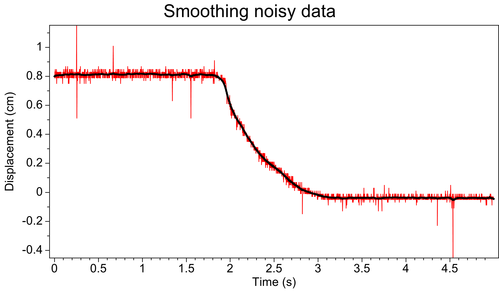
- A noisy input sequence (red) after smoothing (black) with the ten-line program.
Each output value y[i] is a weighted average of
input values x[j].
The weights are proportional to a|i-j|, so
that (for 0 <= a <= 1) they decrease exponentially
with increasing |i-j|.
In this example, the parameter a = 0.932.
In effect, our ten-line program is a smoothing filter.
The weights are normalized so that they sum to one, which means that
when this filter is applied to a sequence with constant input value
x[i] = constant (already as smooth as can be), the output
values will be the same y[i] = constant.
The following figure illustrates weights for the exponential filter and two alternative smoothing filters with comparable widths.
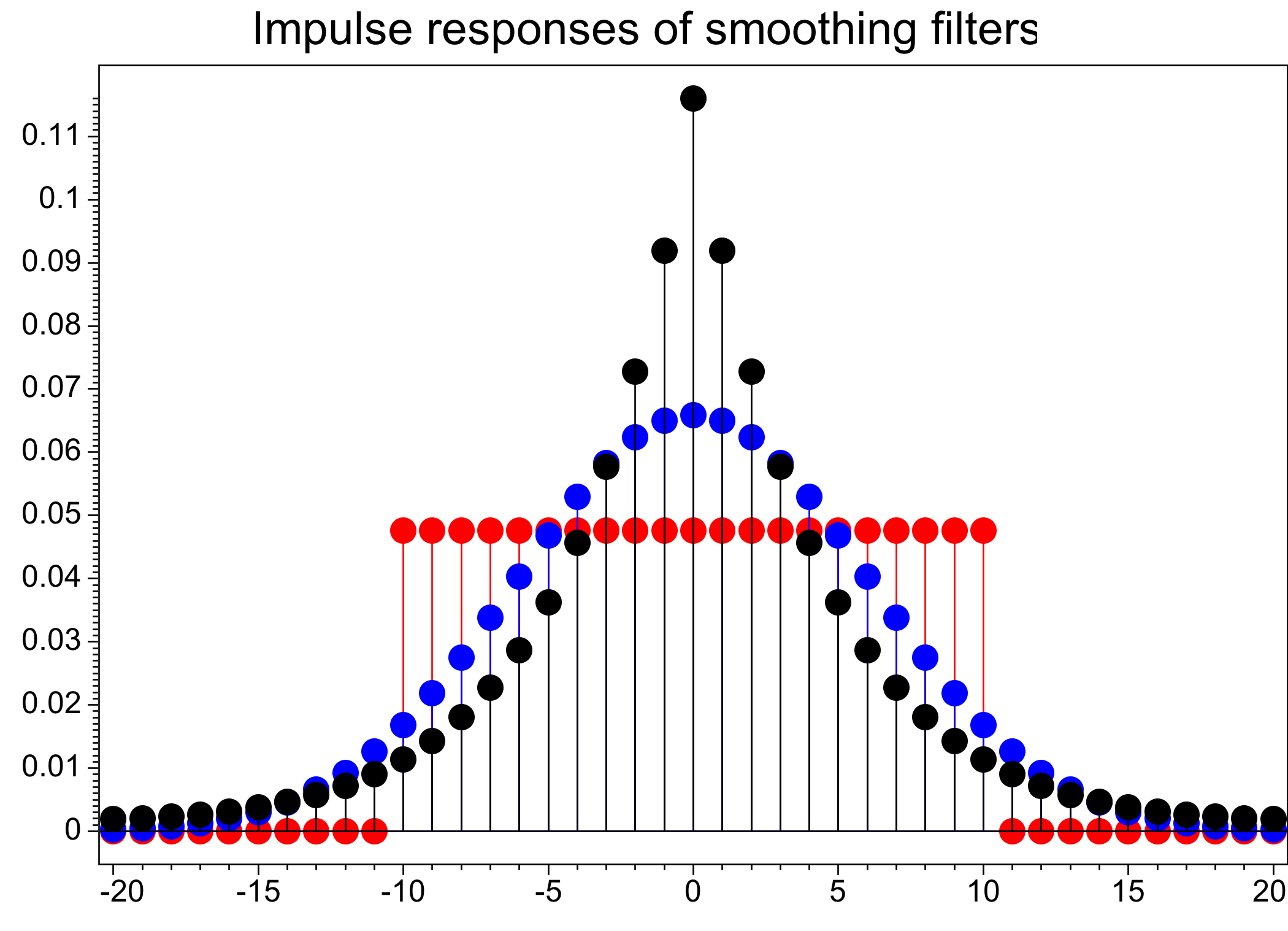
- Impulse responses of exponential (black), Gaussian (blue) and boxcar (red) smoothing filters. For these filters, each output sample is a weighted average of nearby input samples; shown here are the weights.
All three of these smoothing filters can be implemented efficiently, with computational cost that is independent of their width. But efficient (recursive) implementations of both the Gaussian and boxcar filters require more complex programs, especially when carefully handling the ends of input and output sequences.
A less efficient (non-recursive) but simpler implementation of the boxcar filter is often used, perhaps because it more obviously computes a moving average. But the abrupt transition from non-zero weight to zero weight makes no sense for such an average, and it is hard to beat the simplicity of our ten-line program.
To summarize, the exponential filter
- gives more weight to input samples located (in time or space) near the output sample than to input samples located farther away
- guarantees that all weights are non-negative, unlike many recursive implementations of Gaussian filters
-
can be applied in-place, so that output values
y[i]replace input valuesx[i]stored in the same array, which is especially useful when filtering large arrays of arrays that consume a lot of memory -
requires only six floating-point operations (multiplies and adds)
per output sample
y[i], and this computational cost is independent of the extent of smoothing - can be implemented with a simple ten-line computer program that includes careful treatment of the ends of input and output sequences
Careful treatment of the ends is important. When averaging input values to compute output values near the ends, our ten-line program listed above implicitly assumes that input values beyond the ends are equal to the end values. This zero-slope assumption is often appropriate.
Another common assumption is that input values beyond the ends are zero, and the figure below shows how this zero-value assumption may be inappropriate, as the decrease in the output sequence near time zero seems inaccurate.
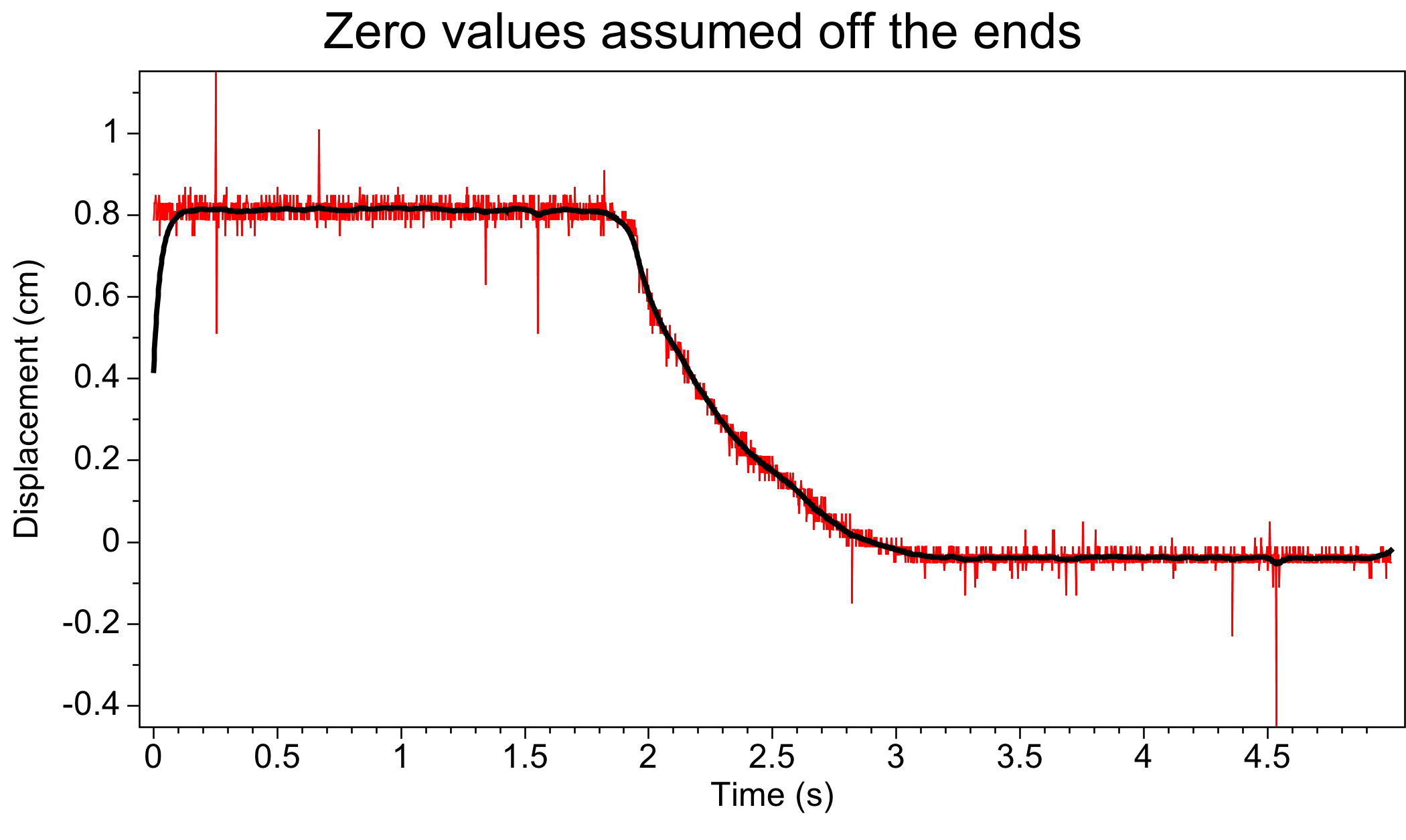
- A noisy input sequence (red) after smoothing (black) with the recursive two-sided exponential filter. Input values off the ends have been assumed to be zero, which seems unreasonable for the left end where times are nearly zero.
But suppose that the data we are smoothing are known to have zero mean. In this case, the zero-value assumption may be more appropriate, and our ten-line program becomes
  float b = 1.0f-a;
  float sx = b, sy = a;
  float yi = 0.0f;
  y[0] = yi = sy*yi+sx*x[0];
  for (int i=1; i<n-1; ++i)
    y[i] = yi = a*yi+b*x[i];
  sx /= 1.0f+a; sy /= 1.0f+a;
  y[n-1] = yi = sy*yi+sx*x[n-1];
  for (int i=n-2; i>=0; --i)
    y[i] = yi = a*yi+b*y[i];
Can you see the difference? It is not obvious, but look carefully at the second line. That's it! A simple change to the initialization of one variable switches our treatment of the ends from zero-slope to zero-value.
One final tip.
The relationship between the extent of smoothing and the
parameter a is not at all intuitive,
so I rarely specify this parameter directly.
Instead, I compute the parameter a to obtain
an exponential filter that (for low frequencies) is comparable to
a Gaussian filter with a specified half-width sigma
(measured in samples), using:
  float ss = sigma*sigma;
  float a = (1.0f+ss-sqrt(1.0f+2.0f*ss))/ss;
So, in practice, this adds two lines to our ten-line program.
And if you would rather think in terms of the integer half-width
m of a boxcar filter, then (again, for low frequencies)
the half-width sigma of the comparable Gaussian filter
can be computed using:
float sigma = sqrt(m*(m+1)/3.0f);
For the boxcar filter with half-width m = 10
displayed in the figure above, these expressions yield
sigma = 6.06 and a = 0.792.
Parallel loops with fork-join
November 28, 2010
Almost five years ago I described a
template for implementing parallel loops
in Java using the standard Java class AtomicInteger.
I have used that template to enhance the performance on multicore
systems of about a dozen loops within the
Mines Java Toolkit.
In doing so I encountered three shortcomings.
First, the boilerplate code required to construct and synchronize threads was lengthy. A loop had to be really important for me to spend the effort writing — usually, I copied, pasted, and modified — that code. Second, it was difficult for me to know how many threads to create in my methods because I could not know how many threads would be created in the methods that called mine. And third, as the number of cores grew — my current workstation has 12 cores, each capable of executing two threads concurrently — the performance of the atomic integer template did not keep up for some loops, especially those with smaller bits of computation inside.
I recently addressed these shortcomings by adding a new class
Parallel to the package edu.mines.jtk.util.
The
online documentation
for Parallel provides some simple examples of
using it to implement parallel loops.
These examples look more or less like this:
Parallel.loop(begin,end,step,new Parallel.LoopInt() {
  public void compute(int i) {
    // some computation that depends on index i
  }
});
Assuming that computations for different loop indices i
are independent, this parallel loop is equivalent to
for (int i=begin; i<end; i+=step) {
  // some computation that depends on index i
}
Here let's use a different example to highlight advantages in
using the new class Parallel for parallel loops.
The matrix multiplication example
To understand the class Parallel and the problems that
it solves, let's consider the following method that computes the
j'th column in a matrix product C = A×B:
static void computeColumn(
  int j, float[][] a, float[][] b, float[][] c)
{
  int ni = c.length;
  int nk = b.length;
  for (int i=0; i<ni; ++i) {
    float cij = 0.0f;
    for (int k=0; k<nk; ++k)
      cij += a[i][k]*b[k][j];
    c[i][j] = cij;
  }
}
For clarity let's ignore various optimizations that we would
normally make within this method, and instead focus on the
method that will call this one, the method with the loop over
j that will compute all of the columns of the
matrix product C.
The simplest loop computes columns of C serially, that is, one after the other:
int nj = c[0].length;
for (int j=0; j<nj; ++j)
  computeColumn(j,a,b,c);
Of course, this single-threaded loop will run no faster on a multi-core system than on a single-core system.
Multithreading with AtomicInteger
One way to speed up this computation on multi-core systems is to execute multiple threads that compute columns of C in parallel. Little synchronization between threads is required, because each column of the matrix product C can be computed independently.
int nthread = numberOfCores();
final int nj = c[0].length;
final AtomicInteger aj = new AtomicInteger();
Thread[] threads = new Thread[nthread];
for (int ithread=0; ithread<nthread; ++ithread) {
  threads[ithread] = new Thread(new Runnable() {
    public void run() {
      for (int j=aj.getAndIncrement(); j<nj;
               j=aj.getAndIncrement())
        computeColumn(j,a,b,c);
    }
  });
}
startAndJoin(threads);
The loop over column index j is almost concealed by the
numerous lines of code required to construct and synchronize threads.
I have reduced the number of lines somewhat by assuming the
existence of some utility methods numberOfCores and
startAndJoin, but this multi-threaded loop is still
much more complex than the serial loop above.
Another complication lies in the use of the standard Java class
AtomicInteger which ensures that only one thread at a
time can get and increment the column index j.
Access to this index is synchronized; and although
AtomicInteger is designed to be fast, this
synchronized access will eventually become a bottleneck for
parallel loops, as the number of threads (cores) increases.
This bottleneck will be most noticeable for small matrices,
for which synchronization time may be a significant fraction
of the time required for multiplication.
Yet another potential source of inefficiency lies in our choice for the number of threads. Suppose that some users of our method for matrix multiplication have many matrix products to compute, and that they are unaware that our method is implemented with multi-threading. They might then call our method in an outer parallel loop over matrix products that is implemented much like our example above. They too will execute multiple threads for their outer loop. If they choose N = number of threads = number of cores, then the composite program will be executing at least N×N threads, all fighting each other for time and memory on N cores.
One solution to this problem of nested parallelism would be to clearly document the fact that our method for matrix multiplication is multi-threaded. This documentation would then serve as a warning to others to not execute threads in outer loops that would compete with ours. Alternatively, we could implement both serial and parallel methods for matrix multiplication, and let users decide which method to use.
Neither solution works well for a toolkit like ours, in which ignorance of implementation is a desirable feature of reusable software components. Although our source code is freely available, we must be able to change the implementation of our methods without causing users of those methods to change their programs.
Multitasking with fork-join
In summary, the three problems I encountered with the atomic integer multi-threading template listed above are (1) software complexity, (2) performance degradation caused by synchronized access to a shared loop index, and (3) excessive thread construction due to nested parallelism.
All three problems are addressed by the new class Parallel.
Using one method and an interface defined within this class, our loop
for matrix multiplication becomes:
int nj = c[0].length;
Parallel.loop(nj,new Parallel.LoopInt() {
  public void compute(int j) {
    computeColumn(j,a,b,c);
  }
});
The method Parallel.loop is overloaded to accept
multiple parameters that describe the indices to be passed to
the method compute defined by the interface
Parallel.LoopInt.
Here, we use the default begin index 0 and the default step 1,
and specify only the end index nj, so that values
j = 0, 1, 2, ..., nj-1 (not necessarily in that order)
will be passed to the method compute.
That method implements the computation performed by the body of
our parallel loop.
In hindsight, I should have written a class like Parallel
long ago to simplify the lengthy atomic integer template listed above.
The method loop in such a class would construct and
synchronize all of the threads, and an internal hidden implemention of
Thread.run would simply pass the atomic integer loop
index j to the user's method compute.
However, the method Parallel.loop does not work this way.
Instead, this method recursively subdivides the specified set of
loop indices into two subsets of indices.
Each subset is represented by a task (not a thread) that is either
split again into two tasks or performed immediately by calling
the user's implementation of compute for each
index within its set.
This recursive subdivision of tasks creates a binary tree of
computation that can be performed efficiently by a
fork-join framework.
That fork-join framework was developed by Doug Lea (1999, Concurrent Programming in Java: Design Principles and Patterns, Addison Wesley; see also A Java Fork/Join Framework ) and is scheduled to be included with Java 7 in 2011. This framework assigns tasks to a pool of threads in a clever way that is designed to keep all threads busy executing the user's compute method, while minimizing overhead and synchronization. Neither threads nor tasks share the loop index, so no synchronized access to an atomic integer is required.
Moreover, before a task splits itself into two smaller tasks, it
first queries the framework for an estimate of the number of excess
tasks already constructed and for which no threads are currently
available to execute them.
If that number exceeds a threshold (say, 6), the task does not split;
rather, it simply performs its computation serially by calling the
user's method compute for each of its loop indices.
This query-before-splitting tactic solves neatly the problem of nested parallelism. Tasks for inner loops will rarely be split when executed by tasks constructed for outer loops, because the outer loops provide sufficient tasks to keep all threads busy.
If not Java, ...
The key to performance in the class Parallel
lies in its focus on tasks instead of threads.
Parallel lets a (soon-to-be standard) Java fork-join
framework construct a shared pool of threads in which tasks can be
executed in parallel.
The same task-based parallelism can be found in frameworks developed
for other programming languages.
For example, the OpenMP standard specifies task-based parallelism via language extensions for C/C++ and Fortran. OpenMP requires a compiler that supports the extensions, but the free GCC (GNU Compiler Collection) does so, as do commercial compilers available from Intel and others.
For C++, Intel provides the
Threading Building Blocks (TBB)
library that is based, in part, on task-based fork-join parallelism.
The TBB library also supports more general patterns beyond loops
for parallel computing, and some of these may be added to the class
Parallel in the future.
Painting images in 3D
January 9, 2010
Decades ago geophysicists and geologists would use colored pencils to paint seismic sections of the earth's subsurface. Those sections were displayed on paper. We would use different colors and shades to represent different geologic layers. Seismic horizons were then simply the boundaries between those colored layers.
So when painting software became widely available with personal computers in the 1980s, it was obvious that we might use this software to interpret seismic images. Digital paint has advantages. It can be applied in multiple overlays that we can easily turn off and on, and mistakes are easy to undo. Moreover, painting geology is simpler and more intuitive and direct than picking seismic horizons. Painted pixels directly represent a model of the subsurface. If we had only 2D seismic sections, we might all be interpreting them in this way.
But as painting software became commonplace, so did 3D seismic images, and no one wants to paint the hundreds or even thousands of 2D seismic sections in a 3D seismic image. So today we pick horizons, the interfaces between geologic entities, instead of painting geology directly.
Imagine that we could paint in 3D
What does this mean? It does not mean painting with perspective on a 2D canvas. That is what artists do. They use perspective and other techniques to give the illusion of 3D. We mean something different. We want to paint voxels (3D pixels) in a 3D canvas (our subsurface model) that coincides with a 3D seismic image.
At the Colorado School of Mines we are blending geophysical image processing and interactive computer graphics to paint in 3D. The key step is to make the orientation and shape of our digital 3D paintbrush conform automatically to features apparent in 3D images. Simple 3D brush shapes like spheres or cubes, analogous to circles and squares found in 2D painting software, will not do.
For as we move our paintbrush along slices of a 3D seismic image, we are actually painting voxels in a 3D subsurface model of the earth. In the example shown here, we are interactively painting all voxels inside the red 3D paintbrush.
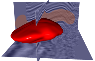
- Painting a 3D seismic image with a 3D paintbrush. As we move the red paintbrush interactively, ...
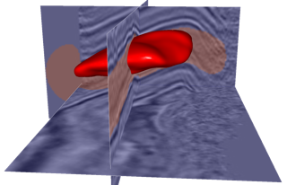
- ... it's shape and size conform automatically to features in the 3D image.
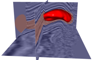
- We paint all voxels within the 3D paintbrush, not only those voxels in the 2D slices displayed here.
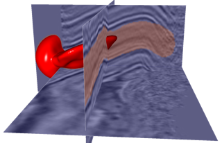
- Where no image is available, as on the left side here, the default brush shape is spherical.
Graphics for manuscripts and presentations
July 5, 2009
Journals require graphics in specific file formats with sufficient resolution and font sizes. For example, the Geophysics Instructions to Authors) specifies:
EPS or TIFF file format.
300-600 dpi (dots per inch) for images,
600-1200 dpi for line art.
If color, then CMYK (not RGB).
8-pt sans-serif fonts for graphic text (e.g., axes labels)
First, which format should we use, EPS or TIFF? For reasons described below, my choice is often neither. Instead I use PNG images, and convert to TIFF only when necessary for publication.
The need for graphics in both manuscripts and presentations raises a second question. Can we use a single graphic in both? For graphics with text, the answer is no. Text in graphics for manuscripts will be too small for presentations. I show below how to compute the correct font size for graphic text.
Which format?
I like image formats. Scalable vector graphic formats like EPS, PDF, and SVG permit unlimited zooming without loss of resolution. In practice, however, no one needs unlimited zooming. A factor of 4 (400% zoom) is almost always sufficient. So we need only ensure that our images have sufficient resolution, not infinite resolution.
Moreover, EPS does not support partial transparency, and none of the vector formats EPS, PDF, or SVG support 3D graphics, such as those generated by OpenGL. So an image format may sometimes be the only option available.
Note that neither of the two formats EPS and TIFF required by Geophysics is supported by the program pdflatex. Instead, pdflatex supports JPEG, PNG and PDF formats. Among these three, I choose the PNG image format for most figures.
The widely used PNG format has lossless compression, honors partial transparency, and can easily be converted to TIFF as necessary for publication. In particular, for color figures, the RGB PNG format can be easily converted to the CMYK TIFF format required by Geophysics.
Image resolution and dimensions
The Mines Java Toolkit (JTK) package edu.mines.jtk.mosaic
can save graphics in PNG format with arbitrary resolution. To facilitate
zooming up to 400%, I save graphics in compressed PNG images with
resolution 720 dpi.
So what figure dimensions - width and height - should we use? Many figures have a natural aspect ratio, so that the height depends on the width, or vice-versa. If we know one dimension, we know the other. For other figures, we may choose width and height independently.
In manuscripts, figure width is usually the limited dimension, because the width of a text column is less than its height. Geophysics allows figures with three different widths, specified in picas. Using 1 pica = 12 pt and 1 inch = 72 pt, these widths are:
1-column = 20 picas = 240 pt ~ 3.33 inches
4/3-column = 26 picas = 312 pt ~ 4.33 inches
2-column = 42 picas = 504 pt ~ 7.00 inches
The 2-column width is not specified in the Geophysics Instructions to Authors, but Geophysics does apparently accept 2-column figures, and they appear to be about 42 picas wide when printed. Both the 1-column and 2-column widths work well with LaTeX styles.
In presentations, figure height is typically more limited than width, because the slide width:height aspect ratio is 4:3 (or higher, for wide-screen formats) and because slides often have a title, which further limits the height available for graphics. Therefore, graphics that fit well in manuscripts may be too tall for slides in presentations. And while we can scale any graphics to fit on a slide, this scaling will always make graphic text too small.
Font size
As noted above, Geophysics requires 8-pt sans serif fonts for graphic text, such as axes labels. Legibility in presentations requires that the font size be at least 1/20 of slide height. These requirements are conflicting.
To see why, suppose that we make a 1-column figure with width 240 pt. If the figure height is also 240 pt, then the 8-pt font size is too small, because 8/240 = 1/30 is less than 1/20 of the graphic height, which cannot exceed the slide height.
The disparity is worse in slides with a title, where graphic height is significantly less than slide height. It is much worse for a two-column figure (again, assuming graphic height = width), for then font size is less than 8/504 = 1/63 of slide height.
The best case occurs when the aspect ratio of our graphic is exactly the 4:3 aspect ratio of a slide. In this case, the graphic height for a 1-column figure in geophysics is 240×3/4 = 180 pt, and the 8-pt font size is approximately 1/22 (~ 8/180) of slide height. By the 1/20 rule, the 8-pt font is almost legible. In fact, a 9-pt font would be perfect for this graphic.
But remember that this is the best case. If we need a title in our slide or change the aspect ratio of the graphic, making it either wider or taller, then the 8-pt font may become much too small for the slide.
Here is an example of the best case, where the graphic has the ideal 4:3 aspect ratio. In this example, the title is part of the graphic image.
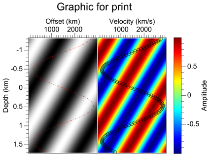
- A graphic with a font suitable for a one-column figure in a printed manuscript. In this best-case scenario, for a 4:3 aspect-ratio, the text is almost large enough for slides.
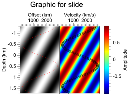
- The same graphic with a slightly larger font that follows the 1/20 rule for slides.
In summary, we should not use the same graphic text for both printed manuscripts and presentation slides. If we do, then graphic text in slides will be too small.
Computing the font size
The Mines JTK creates graphics in on-screen windows, and includes classes with methods to save them in PNG files with higher resolution. It also provides methods that enable the font size to be specified explicitly or computed automatically for either printed figures or slides.
Windows for on-screen graphics can be resized, so that both the width and height of a graphic can be changed interactively. But for any graphic width, it is easy to compute the font size for a figure in a printed manuscript. That is,
fontSizeGraphic = fontSizePrint*widthGraphic/widthPrint
For a 1-column figure in Geophysics,
fontSizePrint = 8 pt and
widthPrint = 240 pt.
For slides, the computation of font size is more complex, in part because not all of the slide width or height may be available for our graphic. Remember that some space may be required for a title or other elements, or we may want to put two graphics on the same slide. So we first introduce two parameters:
widthFraction = fraction of slide width available
heightFraction = fraction of slide height available
We then compute the font size for our graphic window as follows:
widthAvailable = 4*widthFraction
heightAvailable = 3*heightFraction
if widthGraphic*heightAvailable > heightGraphic*widthAvailable:
  heightScale = (heightGraphic*widthAvailable) /
                (widthGraphic*heightAvailable)
else:
  heightScale = 1
fontSizeGraphic = heightGraphic/heightFraction/heightScale/20
The importance of heightScale in this calculation is
not obvious. The purpose of this scale factor is to account for the
decreased height of a graphic placed on a slide when the width:height
ratio of the graphic exceeds that of the space available on the slide.
The complexity of the font size calculation above contributes to the problem of making slides with legible text. I work with folks who all know when text on a slide is too small, but most of them would solve the problem by trial and error. Or they might be safe and always use fonts that are too large. But this simple solution wastes space that might be better used for other content. For example, axes may be necessary in a display of a seismic image, but are usually less important than the image itself.
Indeed, our desire to reserve space for the most meaningful content is the reason that Geophysics specifies a small 8-pt font for text in figures. But, as noted above, this font size is too small for slides used in presentations.
The calculation of font size for slides is tedious without a computer,
and for this reason the class edu.mines.jtk.mosaic.PlotFrame
in the Mines JTK will optionally compute the font size for a slide
(or printed figure) automatically. With this option, as we grow or
shrink the window for an on-screen graphic, the font size grows or
shrinks accordingly.
Making slides and figures (for Mac users)
Given a 720-dpi PNG image with correct font sizes, we must often annotate this graphic by adding additional text, arrows, boxes, and so on. We may also need to create a composite of two or more graphics. I use Apple's Keynote presentation software for Macs to do this.
When making a slide in Keynote, I simply drag a PNG image onto the slide. For presentations I use the default 1024×768 slide size, and so must scale my high-resolution PNG images to fit the space available. I accounted for this scaling in the calculation of font size above, so that any text in the graphic will be legible when presented. I then annotate the graphic using Keynote's drawing tools and, for mathematical symbols and equations, the freely available program LaTeXiT.
Because creating slides for presentations is a visual process, I find that using KeyNote and LaTeXiT in this way is usually more efficient than using the Beamer class with LaTeX. For presentations at technical conferences, I export my KeyNote slides in PDF format.
I also use Keynote when making figures for printed manuscripts. For this purpose, I specify custom slide sizes that conform to print column widths:
1-column = 240 pt = 1200 pixels
4/3-column = 320 pt = 1560 pixels
2-column = 504 pt = 2520 pixels
The Keynote widths in pixels correspond to a resolution of 360 dpi, which is sufficient for precise editing, but half the 720-dpi in our images. That's OK, because Keynote retains the original images, and will preserve their 720-dpi resolution when exporting to a PDF file.
I do not use 720 dpi in Keynote, because the maximum size of a Keynote slide is 4000×4000 pixels. A 2-column figure at 720 dpi is 5040 pixels wide, too wide for Keynote. Also, at 720 dpi, the height of a 1-column figure could easily exceed 4000 pixels. Therefore, I use 360 dpi when annotating print figures in Keynote.
When using Keynote to add text to my figures, I select a font size of 40 pt, because 40 = 8*1200/240 = 8*1560/320 = 8*2520/504. In this way, text that I add to a figure with Keynote is the same size as that in the graphic created with the Mines JTK.
Exporting from Keynote to a PDF preserves the high resolution of any text or other annotation that I add to a figure, as well as the 720-dpi resolution of the graphic images. When I inspect the PDF file using Apple's Preview application, it will have a resolution of 72 dpi, and a large width in inches; e.g., 16.67 inches = 1200/72 for a 1-column figure.
In Apple's Preview (included with Mac OS X), we can save any PDF page as a TIFF (or PNG or JPEG) image with a resolution of 720 dpi. If necessary, with Preview we may also crop the image and, for a color image, convert (match) its RGB color profile to a CMYK color profile.
Apple's support for PDF in Preview is wonderful, but the conversion from PDF to TIFF can be tedious when repeated often as we prepare manuscripts. Therefore, I use a small Python program that exploits Mac OS X services to automate the conversion from PDF to PNG, JPEG, or TIFF.
When preparing drafts, I use low-quality JPEG images, which at 720 dpi, still look sharp, but require far less space than PNG images. Because CMYK TIFF images can be huge, even when compressed, and because pdflatex does not handle TIFF, I use this format only when submitting final figures for a journal like Geophysics.
What's it like to be in geophysics?
January 26, 2008
Dan Shannon is a student-athlete at Grandview Heights High School in Columbus, Ohio. Dan recently asked me some thought-provoking questions:
What do you want your students to get the most out of what you teach (concerning geophysics)?
Most of our students enjoy thinking analytically; they think physics, math, and computer science are fun. I want them to learn how to extend and apply what they already enjoy to design and implement new technology for geophysical exploration, which can be even more fun. In other words, I want my students to develop skills that will enable them to enjoy their work so much that it becomes play, something they might do for only room and board; but they won't because their skills are both rare and valuable.
How do you believe the continued study of geophysics affects the world?
Geophysics enables us to see and better understand the earth's interior. Our ability to do this has many applications. Some geophysicists explore for resources (oil, gas, water, minerals, ...), unexploded ordinance, aging infrastructure in urban areas, ancient civilizations, sites for nuclear waste and CO2 sequestration, and so on. Other geophysicists look much deeper and try to understand geologic processes and forces that cause earthquakes. Or they might use seismic waves generated by earthquakes to better image the earth's core and mantle. This list is far from complete. I should at least mention other planets, and similarities between geophysical and medical imaging. But these are some of the applications of geophysics that have worldwide importance.
What are the unique aspects of geophysical engineering?
The applications described above are rather unique. And perhaps the difference between science and engineering is less well-defined in geophysics. But beyond that, geophysical engineering is much like other engineering fields. For example, I used to think that geophysicists have more opportunities to travel abroad, to see the world. But I have learned by talking with Mines graduates in other engineering fields that many have such opportunities today.
How do the working conditions compare to other jobs; are they indoors, outdoors, both?
Geophysicists work both indoors and/or outdoors. In my geophysical career, I have worked outside covered in drilling mud and inside programming some of the world's fastest supercomputers. Never at the same time, of course, and more of the latter.
What skills can/need to be integrated with geophysical engineering in order to be successful?
In addition to geology and physics (clearly!), successful geophysicists are likely to be skilled in mathematics, computer science, and to a lesser extent chemistry. When I ask my colleagues what subject they wish they had studied more while in school, most of them say math, because that one seems to be most difficult to pick up on the job while solving geophysical problems.
How interpersonal is the study of geophysics?
Probably no more or less so than any other scientific or engineering discipline. But few geophysicists work alone, and many today work in teams with other geoscientists and engineers.
What opportunities does geophysical engineering offer, while in school, that other areas of study do not offer?
The opportunity to learn how mathematics, physics, computer science and geology can all be woven together to do amazing things. Our students tend to be those who enjoy putting these subjects together. Opportunities to work both outdoors, acquiring geophysical data, and indoors, developing and using computer software that analyzes those data, may also be unusual. An example of this is our four-week summer field session, which our students seem to especially enjoy, relative to other students at Mines.
What compels you to be involved in geophysics?
I am more compelled to design and build computer programs, software machines that can be wonderful combinations of art and engineering. Geophysics just happens to provide some of the most challenging computational problems and opportunities. With that interest in computing and an education in physics, I more or less stumbled into geophysics.
What does an ordinary day of work involve?
This varies quite a lot from day to day, but typically includes one or more of the following activities: preparing and teaching classes, working with students, working with colleagues, analytical work for research, writing computer software, writing prose, responding to email, and so on.
What does an extraordinary day of work involve?
A breakthrough in any of the activities listed above followed by a workout with the Mines varsity swimming team with some favorite music running in my brain. So what is a breakthrough? For me that could be working with a student to find a simple and elegant solution to an analytical or computational problem. Or perhaps it is when I am stuck with a programming error while lecturing in a computer science class, and everyone becomes very still (because this rarely happens), and then a student finds the error before I do. Such days are extraordinary.
Tiny displacements in time-lapse seismic images
January 24, 2007
In time-lapse seismic imaging, we often observe displacements of features in images recorded at different times. After accounting for changes in data acquisition, these displacements can be related to compaction of reservoir rocks as fluids are produced from them. We call these displacements apparent shifts because they may be more directly related to changes in seismic wave velocity outside the reservoir than to physical movements of reservoir boundaries.
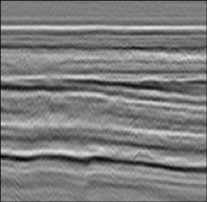
- One of the two seismic images we cross-correlated to detect tiny displacement vectors, one for each image sample.
Today, we typically measure only vertical apparent shifts, for two reasons. First, the force of gravity leads us to expect vertical shifts to be larger than horizontal shifts. Second, it is easier to measure shifts perpendicular to image features than to measure shifts parallel to those features.
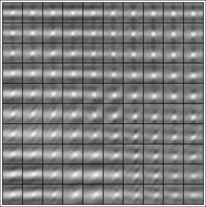
The second problem is illustrated in the figure below, which shows 2-D cross-correlations of local Gaussian windows of two seismic images. The correlation peaks are well resolved vertically, but poorly resolved horizontally. Because the locations of the peaks correspond to the apparent shifts we seek to estimate, horizontal components of those shifts are poorly resolved.
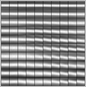
- Local cross-correlations (normalized). This is is a small subset of the correlations that we compute for every image sample. Note the small vertical shifts of some correlation peaks. Horizontal shifts are more difficult to see.
We say "vertical" and "horizontal", when what we really mean is "perpendicular" and "parallel" to features in our images. If those features were dipping at an angle of 45 degrees, then resolution would be equally poor in both horizontal and vertical directions.
Ideally the peaks of our cross-correlations would be isotropic, with roughly the same resolution in all directions, as in the figure below. The processing used here is an example of adapting techniques from general image processing to solve specific problems in seismic imaging. Here we computed so-called phase correlations, and our adaptation is to do this in a seamless way for every sample in our images.
- Local phase correlations (normalized). Again, a small subset of the correlations that we compute for every image sample. Both vertical and horizontal components of shifts can be accurately estimated from the locations of peaks of these phase correlations.
Using phase correlations, we can reliably estimate both vertical and horizontal shifts in time-lapse seismic images with sub-pixel precision. In one example, we have used phase correlations to observe horizontal apparent shifts of about five meters in 3-D images sampled with twenty-five meter trace spacings; and these small sub-sample shifts are correlated with the geometry of the target reservoir.
Our problem now is to analyze these apparent shift vectors, to better understand how they are related to changes within and above producing reservoirs.
Parallel loops with atomic integers
July 29, 2006
A computer you buy today is likely to have multiple cores. A "core" is a CPU that may coexist with other CPUs within a single microprocessor. For example, if you have a dual-processor system with dual-core processors, then you really have a quad-core system, one with essentially four CPUs.
Systems like these are becoming commonplace, because CPUs are not getting faster as they once did. Instead, we are getting more CPUs in a single package.
To take advantage of multi-core computers, we might simply run multiple applications simultaneously. But this solution may be impractical. Sometimes we need a single software application to run faster. In this case, we need to get multiple processors working simultaneously on the same problem within a single application.
Our current situation is summarized well by Herb Sutter, in The Free Lunch is Over: A Fundamental Turn Toward Concurrency in Software (2005, Dr. Dobb's Journal, v. 30, n. 3).
An example
Scientific computing often has outer loops with iterations
that can be performed independently and concurrently.
For example, when computing a matrix product C = A×B, we might
compute each column of the matrix C independently.
Here is some Java code that computes the j'th column of C:
static void computeColumn(
  int j, float[][] a, float[][] b, float[][] c)
{
  int ni = c.length;
  int nk = b.length;
  for (int i=0; i<ni; ++i) {
    float cij = 0.0f;
    for (int k=0; k<nk; ++k)
      cij += a[i][k]*b[k][j];
    c[i][j] = cij;
  }
}
We usually optimize this code by mixing and unrolling these loops, but those optimizations are not relevant here.
To compute the matrix product C, we need only an outer loop over its columns:
int nj = c[0].length;
for (int j=0; j<nj; ++j)
  computeColumn(j,a,b,c);
The problem with this single-threaded program is that it will not run any faster on a quad-core system than it would on a single-core system. Three CPUs may be idle while one does all the work.
Multi-threading
To use all four cores concurrently in a single program, we need multiple threads. We could write the outer loop like this:
int nthread = 4;
final int nj = c[0].length;
Thread[] threads = new Thread[nthread];
for (int ithread=0; ithread<nthread; ++ithread) {
  threads[ithread] = new Thread(new Runnable() {
    public void run() {
      for (int j=0; j<nj; ++j)
        computeColumn(j,a,b,c);
    }
  });
}
startAndJoin(threads);
The last statement calls a utility method that simply starts and
then joins all of the threads in the specified array of threads.
This is easy enough with Java's standard classes
Thread and Runnable.
But this multi-threaded program is no faster!
Each thread maintains it's own loop index j
and will simply duplicate the work of the other three threads.
All four cores will be busy (good) doing the same work
(bad).
Chunky multi-threading
We want different threads to compute different columns. But which columns do we assign to each thread? We could simply divide our outer loop into four chunks, so that each of the four threads computes one fourth of the columns:
int nthread = 4;
int nj = c[0].length;
int mj = 1+nj/nthread;
Thread[] threads = new Thread[nthread];
for (int ithread=0; ithread<nthread; ++ithread) {
  final int jfirst = ithread*mj;
  final int jlast = min(jfirst+mj,nj);
  threads[ithread] = new Thread(new Runnable() {
    public void run() {
      for (int j=jfirst; j<jlast; ++j)
        computeColumn(j,a,b,c);
    }
  });
}
startAndJoin(threads);
This program is better, but is efficient only when all four threads get equal access to the four CPUs. That seldom happens. Threads that finish computing their chunk of columns simply stop working. They do not help other threads complete their chunks. (Have you ever worked with a group like this?) This program is only as fast as its slowest thread.
An atomic outer loop index
A more efficient solution is to have all four threads keep working
until all columns have been computed.
(No one stops working until the job is done.)
Let's have each thread compute the next column not already computed
or being computed.
We do that by letting all four threads share a single outer loop index,
using the standard Java class AtomicInteger:
int nthread = 4;
final int nj = c[0].length;
final AtomicInteger aj = new AtomicInteger();
Thread[] threads = new Thread[nthread];
for (int ithread=0; ithread<nthread; ++ithread) {
  threads[ithread] = new Thread(new Runnable() {
    public void run() {
      for (int j=aj.getAndIncrement(); j<nj;
               j=aj.getAndIncrement())
        computeColumn(j,a,b,c);
    }
  });
}
startAndJoin(threads);
The AtomicInteger aj holds the shared outer loop index
that all threads get and increment.
The name AtomicInteger implies that this
get-and-increment is an indivisible atomic operation,
one that cannot be interrupted or corrupted by another thread
doing the same thing.
With this program, our four threads need not perform an equal amount of work, and all threads continue to run until all of the columns are computed. On an otherwise quiet quad-core system, this program runs approximately four times faster than the single-threaded version.
Moreover, on a single-core system this program is almost as fast
as the single-threaded version.
For large matrices, the extra computation required to launch multiple
threads and get-and-increment an AtomicInteger is negligible.
For small matrices, we might apply the same technique to some other more
outer loop.